Learning to Do Historical Research: Sources
Maps
Visualizing Place, Space, and Time
Brien Barrett
Genya Erling
Introduction
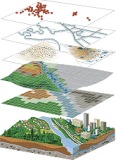
As one of the most useful research tools in environmental history, maps use vivid, visual information to tell vast stories about place, space, and time in a relatively small format. By peeling away the “layers” within maps, you will be able to uncover this valuable information and use it to build and support arguments in your research.
In this section, along with showing you some of the many different kinds of maps available to you, we will guide you to the best places to find these maps. We will also illustrate how to ask important questions about maps and how to use maps to build an argument or as supporting evidence.
Table of Contents
What Kinds of Maps Should You Use?
There are literally hundreds of different kinds of maps that can be used to tell very different stories. One of the first things you need to ask when using maps in your research is: What kind of map will best convey or support my argument?
Decide Which Maps are Best for You
What is your research question?
Be clear in you research question before beginning to look for map evidence. What are you trying to discover about the environmental history of your topic?
What periods are pertinent for your question?
Your question should be narrowed to a specific period. However, some of the systems involved in your question may operate at longer time scales. To gain perspective, it is useful to include information about the area from times before the target date as well.
What systems are involved in your question?
Multiple factors may be playing roles in the environmental processes you are observing. Make a list of the systems likely to be of influence. Many of these systems have spatial components that will be observable using maps. Some examples are:
Building layout/urban form
Transportation
Land forms/topography
Food
Climate
Politics
Race
Economy
Population
Human Health
Industry
Energy
Water
Where are these systems operating?
Now consider your list of important systems. How big are they? How far do they reach? At what scale are they?
Plot
Street
Neighborhood
Town or City
Landscape
Township
County
Watershed
Nation
Continent
Hemisphere
Global
Return to Top of Page
Specific Map Types and Series
Now that you have some idea of what you are looking for, you need some advice on what kinds of maps are available. The following section outlines some specific types of maps that are specifically useful for research in environmental history.
Bird’s Eye Views 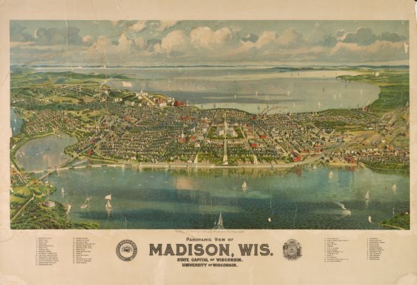
Bird's-Eye View of Madison, 1908, Image ID: WHi-3160, Wisconsin Historical Society
Bird’s-eye views are artists’ renditions of panoramic views of cities drawn from above. In these images, accuracy in details such as street names and locations of important buildings were combined with creative embellishments that can communicate an extraordinarily rich account of the landscape at the time when the map was created. Remember though, these drawings frequently portray an exaggerated prosperity. These images were popular from about 1860 until aerial photography rendered them obsolete in the 1920s.
Period: ~1860 to ~1920
Scale: Neighborhood, Town or City, Landscape
Locations: Urban areas
Systems Present: Urban society, transportation, economy, landforms
Map Sources: Library of Congress; several smaller local collections
Aerial Photography and Orthophotographs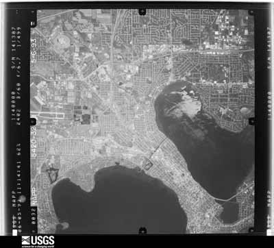
(click for larger version)
NAPP Roll: 5420 Frame: 32 (rotated 0 degrees), U.S. Geological Survey
In the 1930s, aerial photography changed the way we view the landscape. These images provide a real bird’s eye view, and they were used for land surveys after World War I.
Orthophotographs are maps made from aerial photos with corrections made for the angle of the camera with respect to the landscape. Many of these images can be obtained in digital format from the USGS.
Period: 1930s to the present
Scale: Neighborhood, Town or City, Landscape, Township
Locations: Urban areas, Rural Areas
Systems Present: Urban society, Transportation, Economy
Map Sources: Library of Congress; Many sources in state and local collections; Private collections
Plat Maps and Surveyors Notes 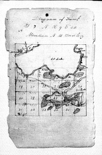
Sketch Map (Dec. 1834) Lyon, Orson INT082E06, Sketch Map, Township 7 North, Range 9 East, Wisconsin Board of Commissioners of Public Lands, and the University of Wisconsin Board of Regents.
Plat maps are based on the Public Land Survey System (PLSS) gridlines that were established as a result of the Northwest Ordinance of 1787. The first surveys were completed in 1820 after the establishment of the US General Office in 1812.
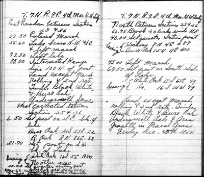
(click for larger version)
Interior Field Notes (Dec. 1834) Lyon, Orson INT082E06, Section Line, Township 7 North, Range 9 East, Between Sections 25 and 26 (North), Wisconsin Board of Commissioners of Public Lands, and the University of Wisconsin Board of Regents.
The original land survey plat maps are enriched with written descriptions of the landscapes included in the surveyor’s notes. This is one of the most important map resources for historical landscape research.
Period: 1820s to Present
Scale: Neighborhood, Town or City, Landscape, Township
Locations: Urban areas, Rural Areas
Systems Present: Landforms, vegetation, landuse, infrastructure
Map Sources: Library of Congress; many sources in state and local collections; Private collections
Return to Top of Page
United States Geological Survey (USGS) Topographic Maps 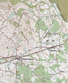
Culpeper County, Virginia, 1992, 1:50,000, Universal Transverse Mercator projection, 49 x 38 inches, U.S. Geological Survey
Topographic maps show landforms and elevation using contour lines. Topographic maps are available at a variety of scales, but the most common are United States Geological Survey 7.5 minute maps, which display areas 7.5 longitudinal minutes by 7.5 latitudinal minutes at a scale of 1:24,000 (1 inch = 2,000 feet).
The United States Geological Survey created the 7.5 minute maps from the time it was created in 1879 until the project’s conclusion in 1992.
Period: 1879 to the present
Scale: Neighborhood, Town or City, Landscape, Township
Locations: Urban areas, Rural Areas
Systems Present: Land forms/topography, building layout/urban form, transportation
Map Sources: Library of Congress; many sources in state and local collections; private collections
Sanborn Fire Insurance Maps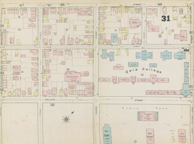
Yale University Library Map Collection, Sanborn 1886, New Haven, Index #31
The Sanborn Fire Insurance Maps are one of the richest and most detailed sources available for historical research in urban areas. The maps were created by the Sanborn Map Company and sold to insurance underwriters for the purpose of assessing risk and determining insurance costs.
The drawings and included key show not only the neighborhood structure and building use, but even specific building information such ceiling height, building materials, and number of stories.
The Sanborn Map Company produced maps in many cities in the United States. They were updated periodically between 1867 and 1950. Use them to observe change over time in urban areas.
Period: 1867 to 1950
Scale: Plot, Street, Neighborhood, Town or City
Locations: Urban areas in the United States
Systems Present: Architecture and urban society, Transportation, Economy
Map Sources: Library of Congress; Wisconsin Historical Society; Yale Map Library; Other local collections
Return to Top of Page
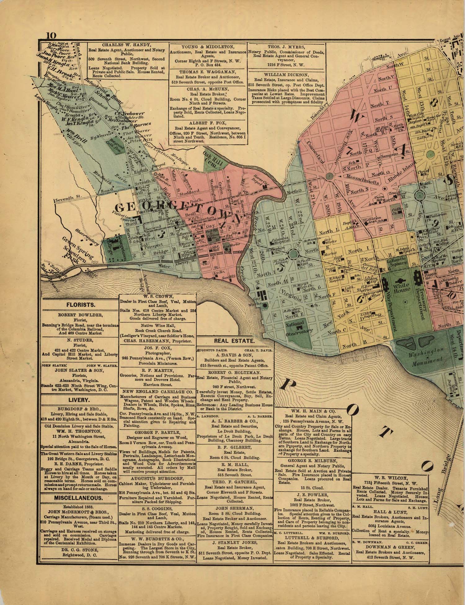
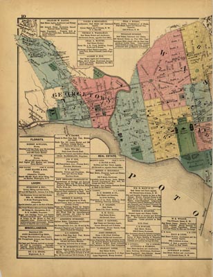
The G. M. Hopkins Company Maps
(click for larger version)
Hopkins, Griffith Morgan. “Atlas of fifteen miles around Washington, including the counties of Fairfax and Alexandria, Virginia / compiled and published from actual surveys by G.M. Hopkins.” Philadelphia, PA. Library of Congress Digital Collections ID: g3850 ct000164.
In 1865, brothers Griffith M. Hopkins and Henry W. Hopkins founded a publishing house in Philadelphia that initially produced county atlases. Over the years, they shifted their focus to city plans and atlases and produced more than 175 city and county atlases for New England, New York, New Jersey, and Pennsylvania.
The G. M. Hopkins Company maps are plat maps that illustrate property owners, structural landmarks (like churches and cemeteries), transportation infrastructure, and bodies of water. This map series also shows dimensions of lots, widths of streets, and names of property owners.
Period: 1867 to 1950
Scale: Plot, Street, Neighborhood, Town or City
Locations: Urban areas in the northeastern United States
Systems Present: Urban form, transportation, economy
Map Sources: Library of Congress, Small local collections – ask your librarian
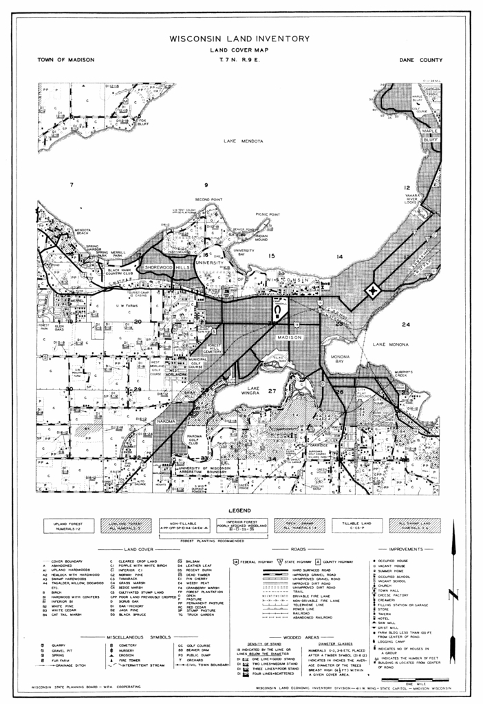
Wisconsin Land Economic Inventory (Bordner Surveys)

(click for larger version)
Town of Madison, Wisconsin Land Economic Inventory (Bordner Survey), 1939, Local ID: EcoNatRes.WILandInv.Dan18.bib, University of Wisconsin Digital Collection.
Beginning in 1929 and running until 1947, the Wisconsin Land Economic Inventory set out to document the current and potential land use in every part of Wisconsin, so areas like abandoned farms and cutover forest could be put to productive use. These maps are useful in that they document the history of the Wisconsin landscape during the Depression era.
Period: 1929 to 1947
Scale: Plot, Street, Neighborhood, Town or City
Locations: Wisconsin
Systems Present: Building layout/urban form, transportation
Map Sources: Wisconsin Historical Society; available through the University of Wisconsin-Madison Digital Collection, Ecology and Natural Resources Collection
Return to Top of Page
These science-based maps contain some of the most concentrated forms of knowledge on single pieces of paper. Available in both historic and current forms, these maps often focus on specific regions and are therefore available from local resources. Ask at local libraries, historical societies, colleges or universities, or government offices for specific sources. Below are a few examples of the many types of thematic maps available.
Soil and Geology
Soil and geologic maps show the geology of an area’s bedrock, sediment, and overall topography and structure of the Earth below the ground. These maps are a valuable resource for research on the processes of Earth, natural resources, and landscape history. 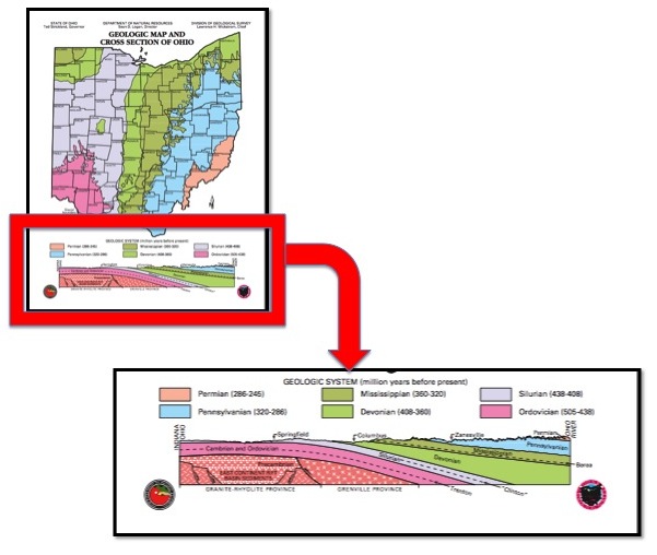
Geologic Map and Cross Section of Ohio, revised 2006, Ohio Department of Natural Resources.
Soil and geologic maps can also come in the form of cross section maps, where a portion of an area (that may or may not be depicted on the map) is taken and shows an area’s general topography and bedrock layering from a side perspective.
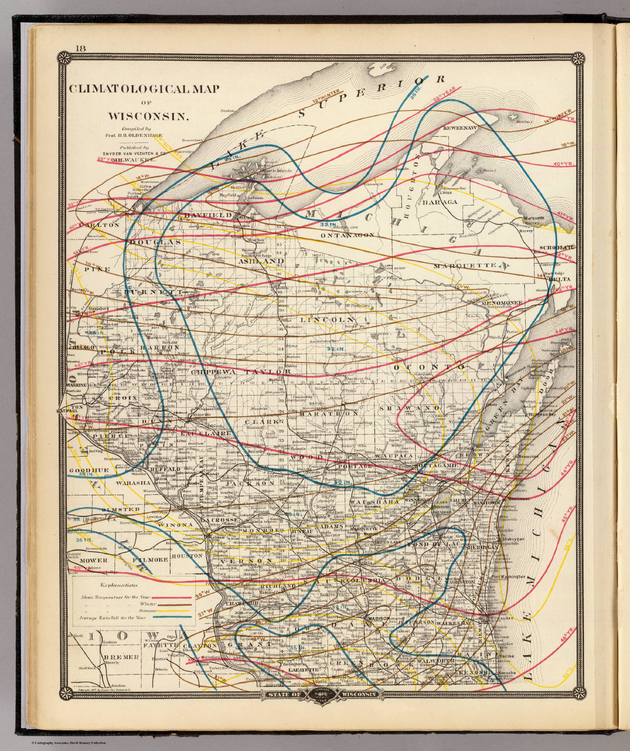
Weather and Climate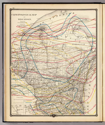
(click for larger version)
Climatological map of Wisconsin. Compiled by Prof. H.H. (sic) Oldenhage. Published by Snyder, Van Vechten & Co., Milwaukee. Copyright 1877, by Snyder, Van Vechten & Co., David Rumsey Collection, Image Number 0936011
Weather and climate maps can be used in ways other than seeing what the weather patterns for the week will be in your local area. These maps show weather and temperature patterns on scales of time that range from hourly to seasonally to yearly. Many historical weather maps show wind patterns and the mean seasonality of temperatures in a selected area.
Vegetation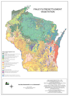
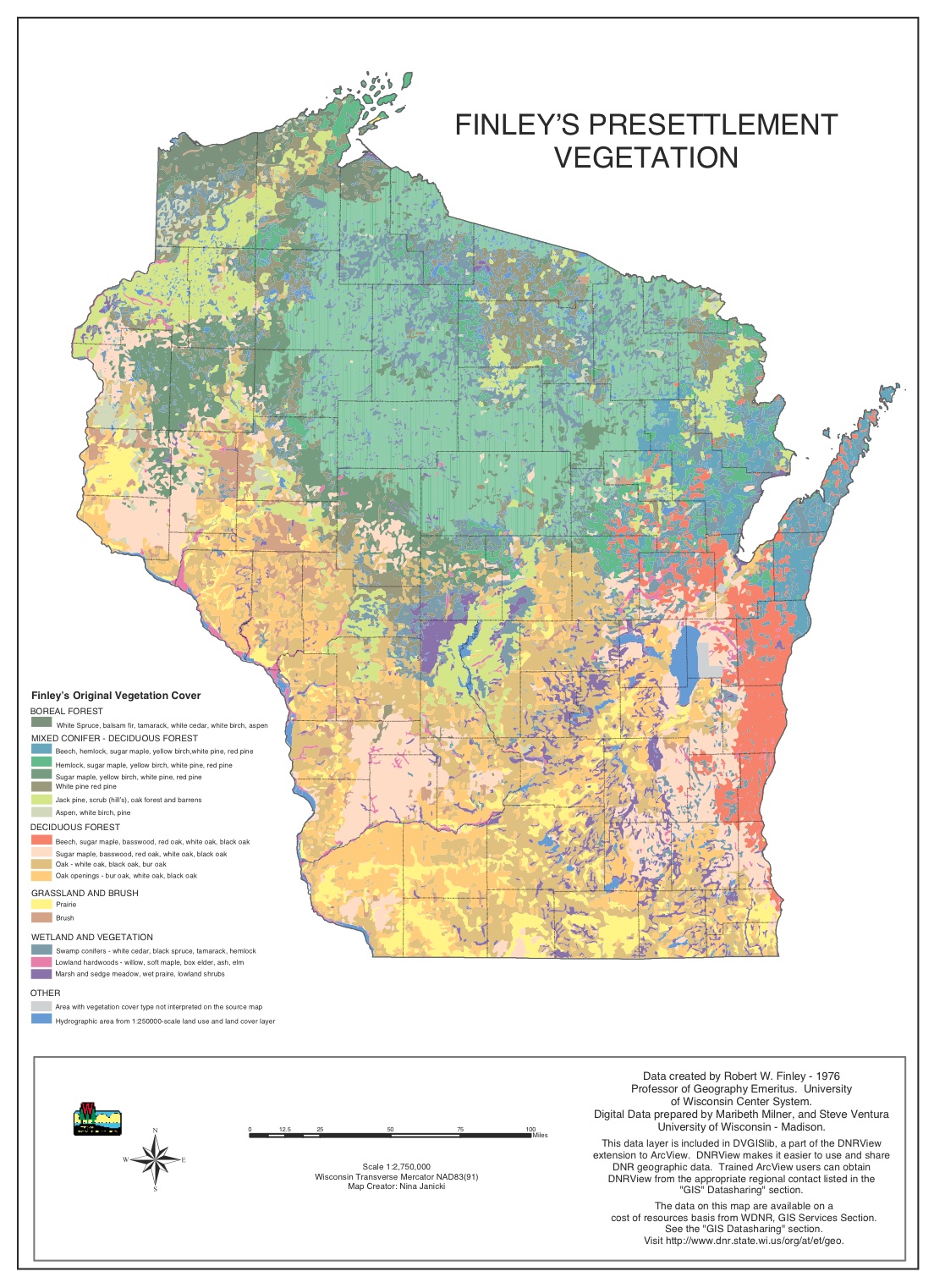
(click for larger version)
Finley’s Presettlement Vegetation, 1976, Wisconsin Transverse Mercator NAD83(91), Wisconsin Department of Natural Resources. This map was distributed in the Ecological Landscapes handbook.
Vegetation maps show the distribution of selected groups of flora across a landscape. They can provide information regarding the natural history of an area and help aid in the reclamation and restoration of regional landscapes.
Infrastructure Maps
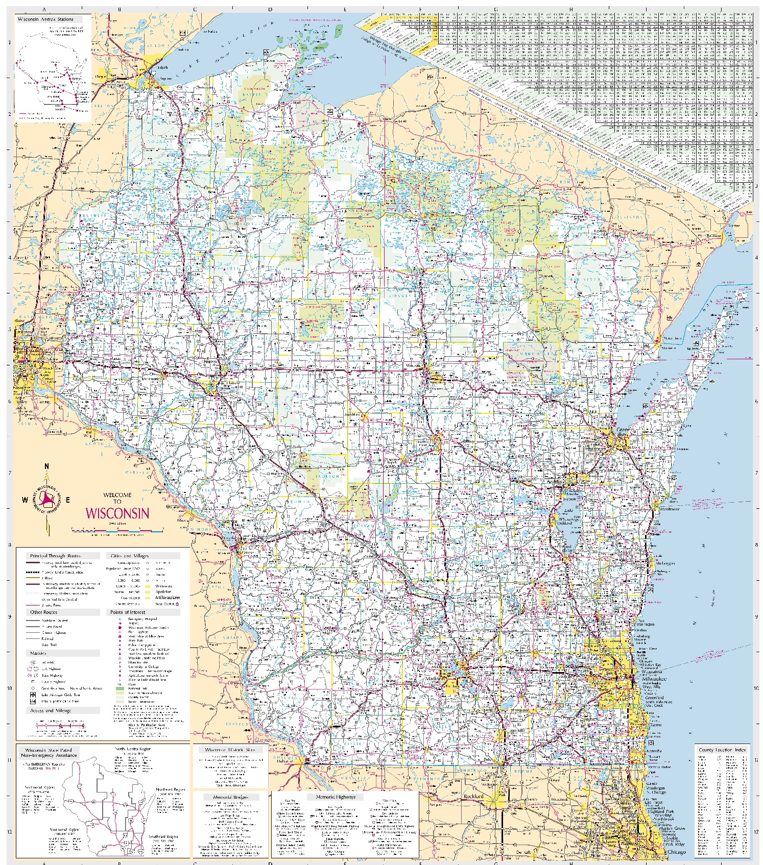
(click for larger version)
“Official Wisconsin State Highway Map,” 2008. Wisconsin Department of Tourism
Infrastructure maps are amongst the most common and easily found maps, as road, railroad, and trail maps can be found in gas stations, train depots, or trailheads. Outlining the location of infrastructure in a certain area, these maps can be of use when observing changes over time and how they are developed in conjunction with real estate trends.
Also consider:
- Landforms
- Land Cover
- Lakes
- Wetlands
- Groundwater
- Floodplains
- Parcel Maps
- Census maps
- School district maps
- Zip code maps
- Utility maps
- Electric Lines
- Sewers
Return to Top of Page
Now that you know some of the different kinds of maps that you can use in your research, you need to know where you can find them. Thankfully, many government agencies, education centers, and private collectors have made millions of maps readily available to researchers. A few important sources are listed below.
The most invaluable resources that you will encounter in your search are the librarians that work at the different locations you visit to get your maps. Be sure to utilize their knowledge early on in the research process, as they can show you short cuts in your research that you may have missed before.
You will also want to consult your professors and librarians about reproducing maps that may be under copyright restrictions.
Library of Congress, Geography and Map Division
- Largest and most comprehensive cartographic collection in the world
- Over 5.2 million maps, including 80,000 atlases, 6,000 reference works, numerous globes and three-dimensional plastic relief models, and a large number of cartographic materials in other formats, including electronic
- Maps date from the fourteenth century to the present
- Large collection of U.S. county and state maps and atlases published in the nineteenth and early twentieth centuries
- Atlases published during the past four or five decades and covering national, regional, state, and provincial
- Excellent collection of manuscript and printed maps of colonial America, the Revolutionary War, the War of 1812, the Civil War, and the wars of the twentieth century.
- Photo-reproductions of manuscript maps from various American and European archives.
- The Hummel and Warner collection includes rare manuscript and printed maps and atlases of China, Japan, and Korea from the seventeenth century.
- Official topographic, geologic, soil, mineral, and resource maps, and nautical and aeronautical charts are available for most countries of the world.
- 700,000 large-scale Sanborn fire insurance maps, in bound and loose sheet volumes.
National Archives and Records Administration, Cartographic and Architectural Section in College Park, Maryland
- Over 15 million maps, charts, aerial photographs, architectural drawings, patents, and ships plans
- Arranged in 190 record groups by specific federal departments and agencies
United States Geological Survey
The US Geological Survey houses an extensive collection of topographic and thematic maps in the following areas:
- United States Maps
- Antarctic Maps
- World Maps
- Planet & Moon Maps
- National Atlas Maps
- National Park Maps
- US Forest Service Visitor Maps
- National Geospatial-Intelligence Agency Foreign Maps
- Hazards Maps
- Geologic Maps
- Other Thematic Maps
- Hydrologic Maps
Office of Coast Survey's Historical Map & Chart Collection, National Oceanic and Atmospheric Administration
- Over 20,000 maps and charts
- Maps dating from the late 1700s to present day
- Collection includes early nautical charts, hydrographic surveys, topographic surveys, geodetic surveys, city plans and Civil War battle maps
Federal Emergency Management Agency
- The FEMA Library is a database of publicly available FEMA resources, including historic flood maps.
Return to Top of Page
Research and Education Institutions
American Geographical Society Collection, University of Wisconsin-Milwaukee
- Over 500,000 maps of all types, including major national topographic series, navigational charts, and thematic maps
- Maps date from 1452 to the present
- Over 200 digital maps, including early maps of Asia, historical maps of many American cities, states, and national parks
Michigan State University Map Library
- ~ 212,000 sheet maps
- 14,000 folded geologic maps
- 4,000 atlases, gazetteers and other reference aids including wall maps, globes, CDs and Internet-accessible resources
- Focus on Michigan, United States, Canada, Africa, Asia, and Latin America
- Maps dating from the 17th to 21st centuries
McGill University Libraries, W. H. Pugsley Collection of Early Canadian Maps
- 6,000 historical maps
- Maps dating from 1556 to the 1940s
- Focuses on the discovery and exploration of Canada and North America, works by sixteenth century European cartographers, and Canadian and Montreal maps from the nineteenth and twentieth century
Newberry Library Maps and History of Cartography Collections
- ~500,000 maps
- Half published before 1900
- Maps from all regions, with a focus on Americas and Western Europe
- Special collections including the Novacco Collection of 16th century maps printed in Italy, the Sack Collection of late 17th and early 18th century maps of western Europe, and the Ayer Collection on the discovery, exploration, and settlement of the Americas
- Extensive collections of maps published by the federal government, county land ownership maps and atlases, General Land Office plats and field notes for Illinois, some 900 maps of the Trans-Mississippi West in the Graff Collection, and the Rand McNally collection of maps and atlases from 1876 to the present
University of Georgia, The Hargrett Rare Book and Manuscript Library
- Over 800 historic maps
- Maps dating from the sixteenth century through the early twentieth century
- Focuses on the State of Georgia and the surrounding region
University of New Hampshire
- ~1,500 JPG-formatted images of historic topographic maps for New York and the New England states.
University of Texas at Austin, Perry-Castañeda Library Map Collection
- Over 250,000 maps covering all areas of the world
- More than 11,000 map images are also available online
University of Wisconsin-Madison, Arthur H. Robinson Map Library
- ~276,000 maps (including topographic, soils, geologic, landuse/landcover, and thematic maps, and nautical and aeronautical charts)
- ~231,700 historic aerial photography images
- ~2,470 aerial photograph mosaic indexes
- ~900 books and other bound volumes including United States gazetteers, atlases, soil surveys, and Wisconsin plat books
- Collection also includes digital geospatial data, digital atlases on CD-ROM, remote sensing imagery, globes, plastic relief models, large wall maps, slides, DVDs, and videocassettes
Wisconsin Historical Society's Map and Atlas Collection
- 25,000 maps and atlases
- Focuses on Wisconsin, the Midwest, the United States, and Canada.
- Most maps date to pre-1900
- The collection includes 17th and 18th century French and British maps of North America, Wisconsin plat maps and atlases, Sanborn
Fire Insurance Company maps for Wisconsin, Wisconsin Bird's-Eye Views, United States General Land Office survey plats and surveyors' notes, Wisconsin topographical maps, military maps, and a wide variety of state, city, county, highway and railroad maps of the United States and Canada
Yale University Library Map Collection
- Over 200,000 map sheets
- 3,000 atlases
- 900 reference books
- ~11,000 rare map prints and manuscripts—generally pre-1850
- Sanborn maps of Connecticut
Return to Top of Page
David Rumsey Historical Map Collection
- 18,460 maps online
- Focuses on rare 18th and 19th century North American and South American maps and other cartographic materials
- Also contains historic maps of the World, Europe, Asia, and Africa
- Collection categories include antique atlas, globe, school geography, maritime chart, state, county, city, pocket, wall, children’s, and manuscript maps.
Many Others
State and Local Resources
- Department of Natural Resources
- Department of Transportation
- Board of Commissioners of Public Lands—Land Records Program
- Local Archives or Historical Societies
- Museums
- Local colleges and other libraries
- Utility companies
- Private commercial businesses
Return to Top of Page
Asking Questions about Maps
By now, you should have a general sense of what maps will be best for your research and where you will be able to find them. However, now that you have your maps, what are you going to do with them? How can a map be beneficial in a research project? What kinds of evidence can be found in maps, and how do you find this evidence?
In the following section, we will break down an 1883 railroad land grant map from the David Rumsey collection. We will show you how to find evidence in the map and how you might use that evidence in your research.
Read the Map. Read Every Word.
When you first lay your eyes on a map, be sure to thoroughly look it over and try to learn as much about the map as possible.
- When was the map made?
- What does it have to say?
- Who was the cartographer?
- What was she/he trying to accomplish by creating this map?
- In your opinion, did she/he succeed?
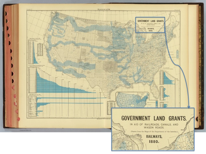
Government land grants, in aid of railroads, canals, and wagon roads. Drawn from the maps of the Department of the Interior. Railways,1880. By Henry Gannett, Published by Charles Scribner's Sons New York. David Rumsey Collection, Image Number 1152177.
The map we are using was produced in 1883 and it showcases land set aside by the federal government in 1880 for use in the construction of railroads, canals, and wagon roads in the United States, along with various inset graphs.
Like any man-made resource, maps can be reflective of the cartographer’s ideological perspectives and biases. Be sure to note that any biases located on the map may not have been purposely included, but are the result of the time and place of which the map was created.
The blue shading located on the main representation of the contiguous United States represents the government land grants, and as you look closer at the map you will notice many interesting features that show a very different United States than the one you know today.
- What is missing from the map that you might see in one that has been created in the past five years?
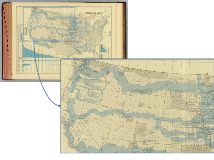
In this particular image, California, Colorado, Iowa, Kansas, Minnesota, Nebraska, and Oregon have received statehood, and Arizona, Idaho, Montana, New Mexico, Utah, Washington, and Wyoming are represented as territories that did not receive statehood until 35 years after the map’s creation. 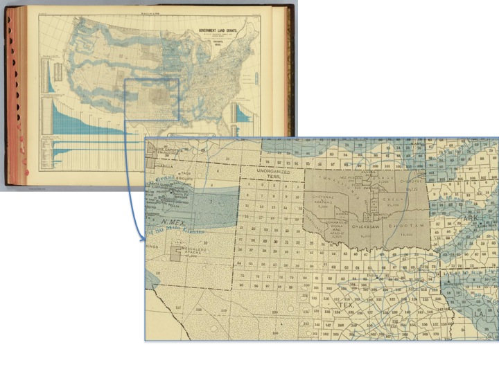
Notice the shades of grey on the previous two sections of the map. These represent Indian territories set aside for use for various native tribes in the American West. Notice how almost the entire state of Oklahoma is assigned as Indian Territory.
- Why would the United States government assign land in Oklahoma as Indian Territory, as opposed to land in the upper Midwest?
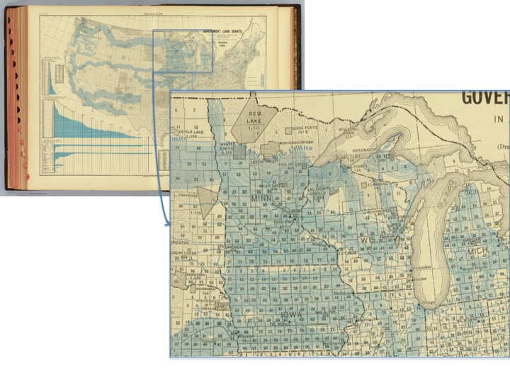
One of the most striking aspects of this section of the map is how much federal land has been set aside for railroads in the Northern Midwest states of Iowa, Michigan, Minnesota, and Wisconsin. If you wanted to illustrate a point that discussed the amount of land received by the railroad companies from the federal government, this section of the map would be a great example to help hammer home your point.
Return to Top of Page
Read the Graphs and Charts
Many maps provide graphs and charts that tell information in supplement to the cartographic aspects of maps.
- What stories do graphs and charts on maps tell in addition to the stories told on the map itself?
- How do these stories relate to the map?
- Why might have the cartographer included these graphs?
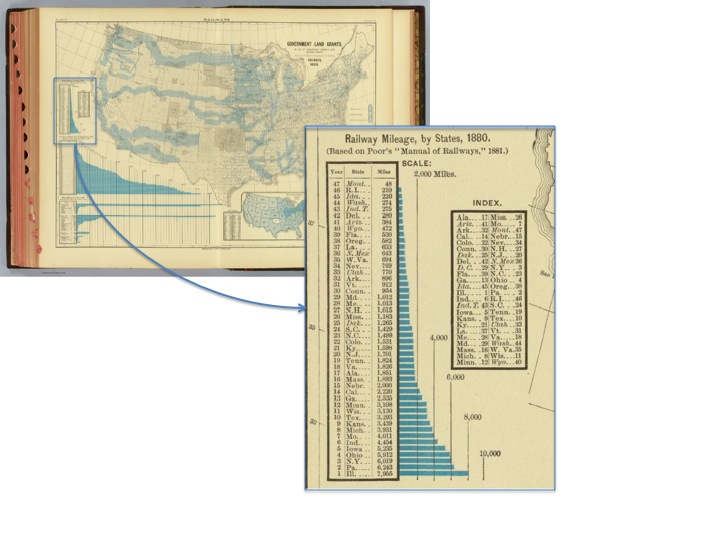
The Government Land Grant map—of which we have been looking—has provided this graph showing the mileage of the railroads in each state.
- What does this graph say about Illinois, New York, and Pennsylvania?
- What types of industries are prevalent in these states that would necessitate such a high amount of railroad tracks?
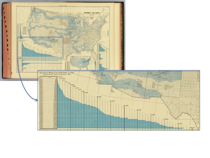
This last image is a graph that shows the total railway mileage of the United States between 1830 and 1880. Within those 50 years, the amount of railroad mileage in the United States increased over 4000 times from 23 miles in 1830 to 93,671 in 1880. When looking at the graph, you can see that despite slow growth in railroad mileage between 1830 and 1850, there is fairly consistent rapid growth between 1850 and 1880. However, in the middle of these 30 years, there is an impediment of growth between 1860 and 1865 before growth grows significantly.
- What would cause this stagnation during the first half of this decade?
- What would be the cause of the large amount of growth following that stagnation?
- Does this graph show any change with the completion of the transcontinental railroad in 1869?
Many maps can contain information that may catch you off guard. In many cases, this can be the richest material to include in your research.
- What about the information caught your eye?
- Does the map tell a different story than what you have learned up to this point?
Return to Top of Page
Using Maps to Make an Argument
For the most part, the main reason why you are looking at sources, like maps, is because you would like to use it to make an argument or help support your argument. Here we will show you examples of how to use a single map to support an argument and how to use multiple maps to help build an argument.
A Single Map to Illustrate Your Point
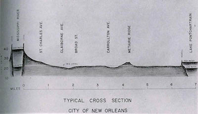
In A River and Its City: The Nature of Landscape in New Orleans, Ari Kelman employs the use of a cross section map to show the various elevation points of New Orleans between the Mississippi and Lake Pontchartrain. In this section of the book, Kelman argues, “Although people founded New Orleans, the city could not have existed without the river. Through dynamic sedimentation, the Mississippi built not only its delta, but also its natural levee…and on the river’s levee New Orleanians built their city.”
Kelman, Ari. A River and Its City: The Nature of Landscape in New Orleans (Berkeley and Los Angeles, CA: University of California Press, 2003, 2006), pp. 21.
Now, take a close look at the New Orleans cross-section map.
- What is striking about the map?
- Where do you think the highest property values are located? How about the lowest?
Kelman then continues, “This topography helps explain part of the waterfront’s significance throughout New Orleans’s history. Rare high ground has always held great value in the city, because prior to the advent of sophisticated draining technologies, the river’s levee provided the only suitable foundation for building in the delta’s soggy environment.”
Kelman’s map serves its purpose in this section of his book brilliantly, as unless you were familiar New Orleans and its various topographic features, you probably would not have had as clear of an idea of what this area looked like. The cross section map provides a vivid understanding of how dependent the city of New Orleans really was on the Mississippi River’s levee during its foundation.
Return to Top of Page
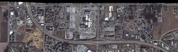
Multiple Maps – Showing Change over Time
The following set of images consists of aerial photos taken over the course of 60 years on Madison’s far-West side. In the fist image, we have highlighted three landmarks for you to use as reference over the set of images:
- The curving bend in the West Beltline Highway of U.S. Route 12,
- James Madison Memorial High School (opened 1966)
- West Towne Mall (opened in 1970)
As you pay attention to these three landmarks in the following series, ask yourself: What impact do these three landmarks have on the landscape as the process of subdivision expands outward from Madison?
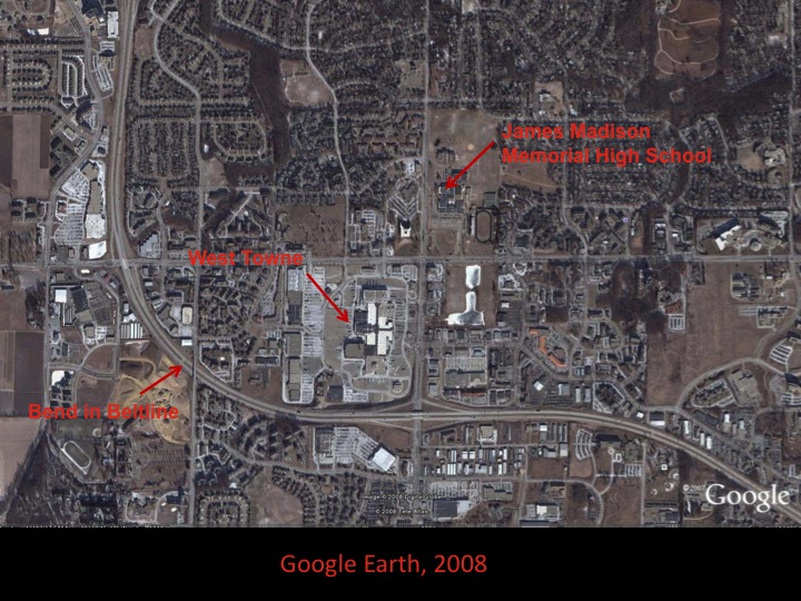
Google Earth
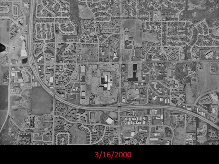
Dane County Land Information Office. “Dane County Wisconsin 2000, 9-16" [aerial photograph]. 1:20,000. Madison, WI: Dane County LIO, 2000.
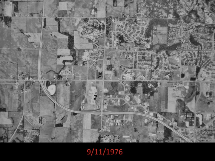
United States Department of Agriculture. "Dane County Wisconsin 1976, USDA 40 55025 276-150" [aerial photograph]. 1:20,000. Salt Lake City, UT: Aerial Photography Field Office, 1976.
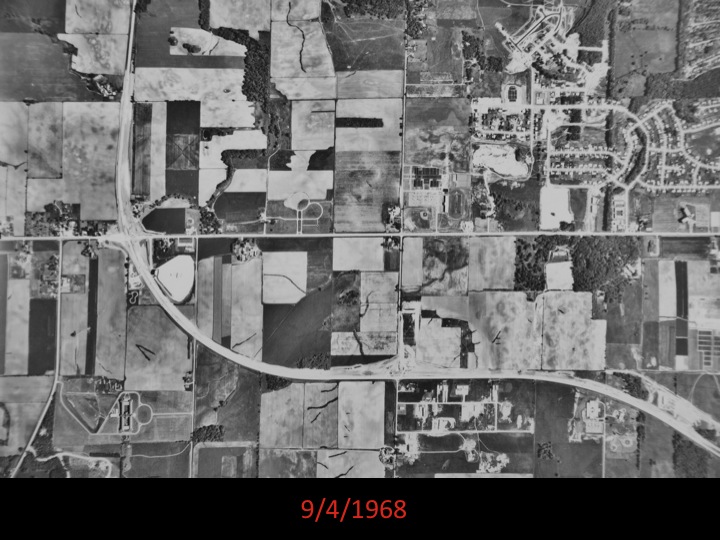
United States Department of Agriculture. "Dane County Wisconsin 1968, WU-3 JJ-55" [aerial photograph]. 1:20,000. Salt Lake City, UT: Aerial Photography Field Office, 1968.
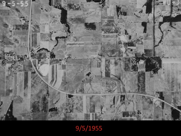
United States Department of Agriculture. "Dane County Wisconsin 1955, WU-3P-34" [aerial photograph]. 1:20,000. Salt Lake City, UT: Aerial Photography Field Office, 1955.
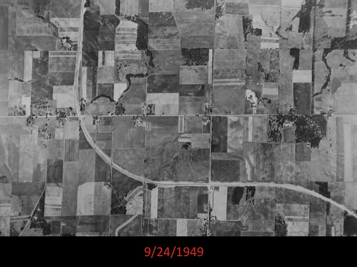
United States Department of Agriculture. "Dane County Wisconsin 1949, WU-2F-19" [aerial photograph]. 1:20,000. Salt Lake City, UT: Aerial Photography Field Office, 1949.
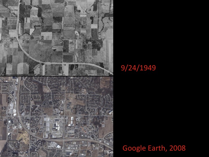
Ask your local library for aerial photographs of your hometown and try to pick out landmarks that are familiar to you. Pay attention to how housing develops around these landmarks, and be sure to ask yourself: Why are the changes I see in these aerial photographs happening?
Return to Top of Page
Querying and Analyzing Maps—Geographic Information Systems
Geographic Information System (GIS) is a tool for analyzing and communicating information. With it, multiple layers of quantitative and spatial data can be stacked on top of each other. With GIS, you can map several features of the landscape at once in order to find patterns. You can also map quantities and densities, and find what’s inside or nearby another geographic location. GIS also allows you to consider all of these data layers over time, so that you can map dynamic processes. GIS is also an important tool for communicating your results.
From ESRI's Guide to GIS: http://www.gis.com/whatisgis/whyusegis.html
Below is a very basic explanation of how to use GIS in environmental history research. For more information, see the glossary at the end of this section, contact your librarian, or explore some of the many on-line tutorials available for GIS instruction. Most college campuses offer training in this technology as well.
Find Your Spatial Data
By now you have identified your question and considered which data sources are available. It is time to put it together. With GIS, census or survey data can be added to historic topographic maps or orthophotographs. First though, you must put the data layers into the geodatabase.
Process Your Data Layers
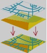
There are several sources for the data layers. Many are already available as digitized maps from universities, private collections, or government offices. At other times, it will be necessary to digitize paper maps, which involves digitally tracing a map to form a set of polygons, thereby creating a vector data layer. At other times, you may need to create raster data layers. This may involve choosing a classification and feature class system to represent your data. Because maps were drawn to different scales and sometimes include significant distortions, you will need to georeference your data layers, aligning them all with a known coordinate system and rubber-sheeting the data layers as necessary.
Use Your Geodatabase to Make an Argument
Now that your geodatabase is established, you can begin to use the information. Again, the explanation below is quite simplified.
Query Your Data Layers
Once you have all of your data layers in your geodatabase, you can begin to ask questions. The GIS software will allow you to isolate areas where features overlap and quantify data within that space. For instance, you could ask the program to find and display all of the areas that were flooded in the aftermath of Hurricane Katrina, and then ask it to quantify the population. With another query you could ascertain the population density of the area, and with yet another, the distance of these areas from emergency evacuation routes.
Communicate Your Results
Now you have the information. The final step is to communicate your results. GIS can be displayed in three different ways: the map view, the database view, or the model view. Each has its benefits and drawbacks, and each will provide unique insight into the system you are observing.
(Much of the information found in this section is based on the helpful guide to GIS, created by ESRI and accessible at www.gis.com/.)
Return to Top of Page
Dos
Do look over your maps very carefully and pay attention to details. Discovering small details in the map could mean striking gold for your research.
Do think about what maps can tell you about the places they depict as well as about the people who made them and the times when they were made.
Do look for maps from local sources.
Don’ts
Don’t forget to site your sources properly. Ask your librarian!
A.H. Robinson Map Library, University of Wisconsin-Madison
ESRI . “Guide to Geographic Information Systems.” www.gis.com/
ESRI. “Online GIS Dictionary.” http://support.esri.com/index.cfm?fa=knowledgebase.gisDictionary.gateway
Library of Congress, www.loc.gov/
United States Geological Survey. www.usgs.gov/
Return to Top of Page
Several parts of this document were inspired and informed by an excellent workshop called Using Geographic Information Systems for Environmental History, which was held at the 2008 Annual Meeting of the American Society for Environmental History.
ESRI . “Guide to Geographic Information Systems.” www.gis.com/
ESRI. “Online GIS Dictionary.” http://support.esri.com/index.cfm?fa=knowledgebase.gisDictionary.gateway
Kelman, Ari. A River and Its City: The Nature of Landscape in New Orleans (Berkeley and Los Angeles, CA: University of California Press, 2003, 2006).
University of Pittsburgh. “Historic Pittsburgh—About Hopkins Plat Maps.” http://digital.library.pitt.edu/maps/mapsexplained.html
Wisconsin Board of Commissioners of Public Lands. “Wisconsin Public Land Survey Records: Original Field Notes and Plat Maps.” http://digicoll.library.wisc.edu/SurveyNotes/
Wisconsin Land Economic Inventory. “The Bordner Survey, Land Cover Maps.” http://steenbock.library.wisc.edu/bordner/
Wisconsin Historical Society. “Sanborn Fire Insurance Company Maps.” www.wisconsinhistory.org/libraryarchives/maps/sanborn.asp
Wisconsin State Cartographer’s Office. “Maps.” www.sco.wisc.edu/maps/maps.php
Return to Top of Page
All definitions and glossary images in this section are from ESRI’s GIS Dictionary:
(http://support.esri.com/index.cfm?fa=knowledgebase.gisDictionary.search&search=true&searchTerm=coverage)
Attribute: 1. Nonspatial information about a geographic feature in a GIS, usually stored in a table and linked to the feature by a unique identifier. For example, attributes of a river might include its name, length, and sediment load at a gauging station. 2. In raster datasets, information associated with each unique value of a raster cell. 3. Information that specifies how features are displayed and labeled on a map; for example, the graphic attributes of a river might include line thickness, line length, color, and font for labeling. 4. In MOLE, a spatial information about a geographic feature in a GIS, usually stored in a table and linked to the feature by a unique identifier. For example, attributes of a force element might include its name and speed. Most MOLE attributes are what some military specifications refer to as labels or modifiers.
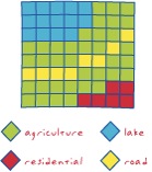
Classification: The process of sorting or arranging entities into groups or categories; on a map, the process of representing members of a group by the same symbol, usually defined in a legend.
Digitizing: The process of converting the geographic features on an analog map into digital format using a digitizing tablet, or digitizer, which is connected to a computer. Features on a paper map are traced with a digitizer puck, a device similar to a mouse, and the x,y coordinates of these features are automatically recorded and stored as spatial data.
Feature Class: In ArcGIS, a collection of geographic features with the same geometry type (such as point, line, or polygon), the same attributes, and the same spatial reference. Feature classes can be stored in geodatabases, shapefiles, coverages, or other data formats. Feature classes allow homogeneous features to be grouped into a single unit for data storage purposes. For example, highways, primary roads, and secondary roads can be grouped into a line feature class named "roads." In a geodatabase, feature classes can also store annotation and dimensions.

Geodatabase: A database or file structure used primarily to store, query, and manipulate spatial data. Geodatabases store geometry, a spatial reference system, attributes, and behavioral rules for data. Various types of geographic datasets can be collected within a geodatabase, including feature classes, attribute tables, raster datasets, network datasets, topologies, and many others. Geodatabases can be stored in IBM DB2, IBM Informix, Oracle, Microsoft Access, Microsoft SQL Server, and PostgreSQL relational database management systems, or in a system of files, such as a file geodatabase.
Georeferencing: Aligning geographic data to a known coordinate system so it can be viewed, queried, and analyzed with other geographic data. Georeferencing may involve shifting, rotating, scaling, skewing, and in some cases warping, rubber sheeting, or orthorectifying the data.
Layer: The visual representation of a geographic dataset in any digital map environment. Conceptually, a layer is a slice or stratum of the geographic reality in a particular area, and is more or less equivalent to a legend item on a paper map. On a road map, for example, roads, national parks, political boundaries, and rivers might be considered different layers.
Overlay: 1. A spatial operation in which two or more maps or layers registered to a common coordinate system are superimposed, either digitally or on a transparent material, for the purpose of showing the relationships between features that occupy the same geographic space. 2. In geoprocessing, the geometric intersection of multiple datasets to combine, erase, modify, or update features in a new output dataset.
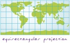
Projection: A method by which the curved surface of the earth is portrayed on a flat surface. This generally requires a systematic mathematical transformation of the earth's graticule of lines of longitude and latitude onto a plane. Some projections can be visualized as a transparent globe with a light bulb at its center (though not all projections emanate from the globe's center) casting lines of latitude and longitude onto a sheet of paper. Generally, the paper is either flat and placed tangent to the globe (a planar or azimuthal projection) or formed into a cone or cylinder and placed over the globe (cylindrical and conical projections). Every map projection distorts distance, area, shape, direction, or some combination thereof.
Raster: A spatial data model that defines space as an array of equally sized cells arranged in rows and columns, and composed of single or multiple bands. Each cell contains an attribute value and location coordinates. Unlike a vector structure, which stores coordinates explicitly, raster coordinates are contained in the ordering of the matrix. Groups of cells that share the same value represent the same type of geographic feature.
Rubber-sheeting: A procedure for adjusting the coordinates of all the data points in a dataset to allow a more accurate match between known locations and a few data points within the dataset. Rubber sheeting preserves the interconnectivity between points and objects through stretching, shrinking, or reorienting their interconnecting lines.
Scale: 1. The ratio or relationship between a distance or area on a map and the corresponding distance or area on the ground, commonly expressed as a fraction or ratio. A map scale of 1/100,000 or 1:100,000 means that one unit of measure on the map equals 100,000 of the same unit on the earth. 2. In reference to double precision, the number of digits to the right of the decimal point in a number. For example, the number 56.78 has a scale of 2.
Symbology: The set of conventions, rules, or encoding systems that define how geographic features are represented with symbols on a map. A characteristic of a map feature may influence the size, color, and shape of the symbol used.
Thematic Map: A map designed to convey information about a single topic or theme, such as population density or geology.
Topology: 1. In geodatabases, the arrangement that constrains how point, line, and polygon features share geometry. For example, street centerlines and census blocks share geometry, and adjacent soil polygons share geometry. Topology defines and enforces data integrity rules (for example, there should be no gaps between polygons). It supports topological relationship queries and navigation (for example, navigating feature adjacency or connectivity), supports sophisticated editing tools, and allows feature construction from unstructured geometry (for example, constructing polygons from lines).
Vector: A coordinate-based data model that represents geographic features as points, lines, and polygons. Each point feature is represented as a single coordinate pair, while line and polygon features are represented as ordered lists of vertices. Attributes are associated with each vector feature, as opposed to a raster data model, which associates attributes with grid cells. 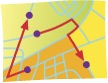
Return to Top of Page
|